
Hypothesis Testing and Minimax Framework
Hypothesis Testing
Introduction
Hypothesis testing is an fundamental tool in statistics for building a complete and scientific procedure to identify our beliefs about the world and evaluate the errors in our conjectures. Typically, the core of a hypothesis testing procedure consists of two statements:
\[\begin{aligned} H_0 &: \text{A belief about something};\\ H_1 &: \text{Another belief}. \end{aligned}\]$H _{0}$ is called the null hypothesis, while $H _{1}$ is called the alternative hypothesis. We require that $H _{0}$ and $H _{1}$ are at least mutually exclusive to precisely convey the testing analysis. For example, good $H _{0}$ and $H _{1}$ can be “There will be no rain tomorrow” and “There will be rain tomorrow”, or “The vaccine is not effective” and “The vaccine is effective”. In contrast, “Tomorrow will be sunny sometime” and “Tomorrow will be rainy sometime” are bad $H _{0}$ and $H _{1}$, since both statements can be true at the same time and therefore it is hard to distinguish them.
Testing Functions
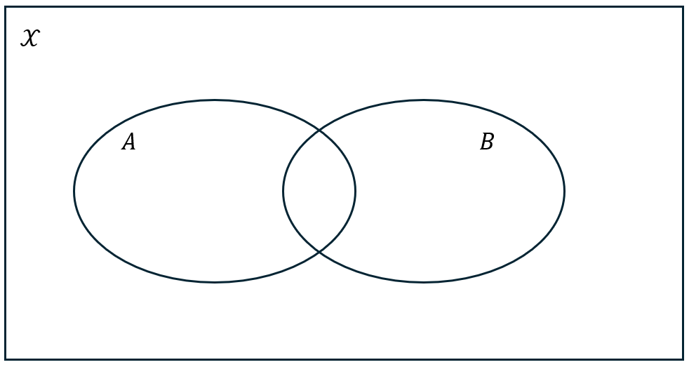
Once the hypothesis are designed, statisticians need to do another important thing — design a testing function. Rigorously speaking, a testing function in hypothesis testing is a mapping from the sample space $\mathcal{X}$ to the decision space $\left\{ 0,1 \right\}$: $T(\cdot): \mathcal{X}\mapsto \mathcal{A}=\left\{ 0,1 \right\}$, where 1 typically represents rejecting the null hypothesis $H_0$ and 0 represents failing to reject the alternative hypothesis $H_0$. Why instead of saying “accept $H_1$”, we say “failing to reject $H_0$”? This is a philosophy question! Note that the testing function $T(\cdot)$ should only depend on the observed data $X \in \mathcal{X}$, and should not depend on any unknown information such as the parameters of the true distribution $\mathcal{P}$ that $X$ is drawn from! (Otherwise, you are actually cheating!) The conditions required for hypothesis statements and testing function are actually very mild, and therefore the hypothesis and the testing function can be very general and flexible.
Errors of Testing
Due to the limit of our knowledge, information and ability to infer, our testing function is not always accurate. There are two types of errors in hypothesis testing:
• Type I error: the testing function rejects the null hypothesis $H _{0}$ when actually $H _{0}$ is true;
\[ \text{Type I error}=\mathbb{P}_{\theta _{0}}(T(X)=1), \theta _{0}\in H _{0}. \]
• Type II error: the testing function fails to reject the null hypothesis $H _{0}$ when actually $H _{1}$ is not true.
\[ \text{Type II error}=\mathbb{P}_{\theta _{1}}(T(X)=0), \theta _{1}\in H _{1}. \]
| Prediction: $H _{0}$ | Prediction: $H _{1}$ | |
|---|---|---|
| Reality: $H _{0}$ | Correct | Type I Error (False Positive) |
| Reality: $H _{1}$ | Type II Error (False Negative) | Correct |
In most statistical models, to relieve ourselves and simplify the analysis, we assume that our probability model is parametric, i.e., the true distribution $\mathcal{P}$ is indexed by a parameter $\theta \in \varTheta $. Under this assumption, we can rewrite $H _{0}$ and $H _{1}$ as
\[\begin{aligned} H_0 &: f (\theta ) \in R _{1};\\ H_1 &: f (\theta ) \in R _{2} \end{aligned}\]for some function $f$. Such $f$ can be various. For example, it can be the expectation/variance of $f _{\theta }(x)$, or the maximum density or probability mass: $f=\max\limits _{x \in \mathcal{X}}f _{\theta }(x)$, etc, anything interested! Note that our assumption of separation requires that $R _{1} \cap R _{2} = \varnothing$. For simplicity, let’s first assume that our hypotheses are simple, which means $f$ is the identity and $R _{1},R _{2}$ only consist of a single element:
\[\begin{aligned} H_0 &: \theta =\theta _{0};\\ H_1 &: \theta =\theta _{1}. \end{aligned}\]Significance Level and Risk Function
Let’s first define the power function of a testing function given the parameter $\theta $ of the distribution:
For most of non-trivial hypothesis testing problem, it is impossible to design a perfect testing function that has both zero Type I and Type II errors. (However, things are not that bad, because it is also impossible to design a testing function that is a total trash — always making mistakes! Why?) The word “both” is important, because we can trivially achieve zero Type I error by never rejecting $H _{0}$, and achieve zero Type II error by always rejecting $H _{0}$. In other words, to design a good testing function, we should not reduce one type of error simply by sacrificing the other type of error. To balance the two types of errors of a test $T$, we can try to minimize the weighted sum of the two errors, i,e.,
\[ R(T)=\omega \cdot \text{Type I error}+(1-\omega )\cdot \text{Type II error}=\omega \mathbb{P} _{\theta _{0}}(T(X)=1)+(1-\omega )\mathbb{P} _{\theta _{1}}(T(X)=0). \]
Such risk can be regarded as putting a prior $\pi $ on the parameters $\theta _{0}$ and $\theta _{1}$: $\mathbb{P} _{\pi }(\theta =\theta _{0})=\omega $, $\mathbb{P}(\theta =\theta _{1})=1-\omega $. When $\omega =\frac{1}{2}$, such risk function can be viewed as an expected loss of the testing function $T$ with the 0-1 loss $l(T)=\mathbf{1} _{\left\{T(X)=f(\theta )\right\}}$.
Neyman-Pearson Framework
A good strategy to select useful testing functions to first fix an upper bound $\alpha $, limit our scope on the testings with Type I error less than $\alpha $, and see how small we can make the Type II error within the scope. The $\alpha $ here is called the significance level of the testing function. In other words, if we define $A _{s}(\mathcal{P} _{\theta },\alpha )$ as the set of all testing functions that have Type I error no larger than $\alpha $, then we want to solve the following problem:
Such approach is called the Neyman-Pearson Framework. The optimization problem above is not easy in general. However, when $H _{0}$ and $H _{1}$ are simple hypotheses, surprisingly and beautifully, we have very intuitive solution and it is optimal in some sense.
• For any testing function $T \in A _{s}(\mathcal{P} _{\theta },\alpha )$, $T ^{\star }$ always has smaller Type II error: $\mathbb{P} _{\theta _{1}}(T(X)=0) \ge \mathbb{P} _{\theta _{1}}(T ^{\star }(X)=0)$;
• Any testing function of a UMP level test must be of the form of $T ^{\star }$ except on a set of measure zero under $\mathbb{P} _{\theta _{0}}$ and $\mathbb{P} _{\theta _{1}}$.
ROC Curve
We have Type I and Type II errors to evaluate the performance of a testing function. However, we are still not satisfied with these mere two numbers. Is there any way to illustrate a testing function more intuitively and visually? In this view, the receiver operating characteristic (ROC) curve is a good choice! However, the ROC curve is not applied to a single testing function, but rather a family of them. Typically, a testing function is fixed somehow, meaning that we have a raw function inside the testing function and a threshold $c$ to determine the final decision. For example, in the Neyman–Pearson lemma, the raw function is the likelihood function $L(X)$, and the threshold is $k$. In this way, the Type I and II errors are fixed. In the ROC curve, instead, we give the testing function “more freedom” by allowing the threshold to vary. These, definitely, will change the Type I and II errors. If we draw the plot of the Type I error (x-axis) and the power under $H _{1}$ (y-axis) as the threshold varies, this is the ROC curve!

The x-axis of the plot is the “false positive rate”, which means “among all of the cases in $H _{0}$, how many are wrongly detected as $H _{1}$?”, which is exactly the Type I error; the y-axis is “among all of the cases in $H _{1}$, how many are correctly concluded?”, which is $1-\text{Type II error}$. The line connecting $(0,0)$ and $(1,1)$ represents the random guess (since we are guessing randomly, the probability of concluding $H _{1}$ is the same under both $H _{0}$ and $H _{1}$). The very left top corner represents the perfect test, which has zero Type I and Type II errors. This perfect test, however, rarely exists. As long as any $\mathbb{P}$ in $H _{0}$ and $\mathbb{Q}$ in $H _{1}$ has positive total variation distance, i.e., $\max\limits _{\mathbb{P}\in H _{0},\mathbb{Q}\in H _{1}}\text{TV}(\mathbb{P},\mathbb{Q})>0$, then such perfect test does not exist. In this plot, every curve starts at $(0,0)$ (representing that it never rejects $H _{0}$, and therefore cannot correctly detect any case in $H _{1}$ either), and ends at $(1,1)$ (representing that it always rejects $H _{0}$, and therefore wrongly rejects all the cases in $H _{0}$). Additionally, the closer the curve is to the top left corner, the better the testing function is. If one curve is always above another curve, then the testing function corresponding to the upper curve is better than the other one. The area under the curve (AUC) is roughly a summary of the performance of the testing function. An area close to $1$ means that the testing function is very accurate, while an area close to $0.5$ means that the testing function is as bad as random guess. These properties of ROC can be easily verified by the definition of the ROC curve and the plot.
$F$-$1$ Score
$F$-$1$ score is also a popular evaluation for a testing function, where $F$-1 score is defined as \[ F\text{-}1 = \frac{2}{\frac{1}{\text{precision}}+\frac{1}{\text{recall}}}=\frac{2\cdot \text{precision}\cdot \text{recall}}{\text{precision}+\text{recall}}, \]
where precision and recall are defined as
In other words, precision measures “in all of predicted positive cases, how many are actually positive”. Low precision means the overlap of the predicted positive cases and the actual positive cases is small compared to the size of the predicted positive cases — there are many false alarms. Recall measures “in all of actual positive cases, how many are predicted positive”. Low recall means among the actual positive cases, most are missed by the testing funciton. Both low precision and low recall are undesirable, and will lead to poor $F$-$1$ score. (Why is $F$-$1$ score not defined as the arithmetic mean of precision and recall?) Note that the roles of the actual postive cases and the predicted positive cases are not symmetric in the definitions of precision and recall, which provide a good reason to explain why typically the testing problem is not equivalent when we exchange $H _{0}$ and $H _{1}$.
Multiple Parameters
The measures mentioned above is only for a single parameter $\theta \in \varTheta$. However, since usually we do care about a hypothesis that contains a set of parameters, how to evaluate the performance of a testing function in this case?
For example, if we assume that the data are drawn from a Guassian distribution, then the distribution can be parametrized by the mean $\mu$ and the standard deviation $\sigma$, and hence $\varTheta =(\mu, \sigma), \mu \in \mathbb{R}, \sigma>0$. Similarly, if we assume that the data are from a multinomial distribution with $k$ categories, then the distribution can be parametrized by the probabilities of each category $p_{1},\dots,p_{k}$, subject to the constraint that $\sum\limits_{i=1}^{k}p_{i}=1$. In this case, $\varTheta =\left\{(p_{1},\dots,p_{k}): \sum\limits_{i=1}^{k}p _{i}=1, p _{i}\ge 0 \right\}$, i.e., a simplex in $\mathbb{R}^{k}$.
In the example above, what can you conclude about the Type II error for general $p \neq 0.5$?
Prior of the Parameters
If we have a prior distribution $\pi $ on the parameter space $\varTheta $ (as is the case in Bayesian statistics), then a natural way is to “take the average” of the risk function over $\varTheta $. For a given testing function $T(\cdot )$, we have a risk function $r(\theta ,T(\mathbf{X}))$, which measures the error of $T$ for each sample $\mathbf{X}$ from $\mathbb{P} _{\theta }$ (for example, the Type I error when $H _{0}$ holds or the Type II error when $H _{1}$ holds). If we take the expectation of $r(\theta ,T(\mathbf{X}))$ over $\mathbf{X}$, we get a quantity $R(\theta ,T)=\mathbb{E} _{\mathbf{X}}r(\theta ,T(\mathbf{X}))$, which is only a function of $\theta $ and irrelevant to the samples. If we continue taking the expectation over $\theta $, we get the Bayes risk of $T$ as
The testing function that minimizes the Bayes risk is called the Bayes test.
Such Bayes risk can actually be defined beyond the testing problem. For any decision problem with a decision function, as long as we have a risk function, we can define the Bayes risk by taking the corresponding expectation. For example, in the estimation problem, the decision function is an estimator $\hat{\theta }$ that aims to provide a good estimation of the true parameter $\theta $. The estimator that minimzes the Bayes risk is called Bayes estimator. A common selected risk function is the mean square error (MSE): $R(\theta ,\hat{\theta })=(\hat{\theta }-\theta )^{2}$. If we denote the prior of $\theta $ as $\pi (\theta )$, then we have \[ R(\theta ,\hat{\theta })=\displaystyle\int_{\varTheta }^{}\displaystyle\int_{\mathcal{X}}^{}(\hat{\theta }-\theta )^{2}f(x|\theta )\pi (\theta )dx d\theta =\displaystyle\int_{\mathcal{X}}^{}\displaystyle\int_{\varTheta }^{}(\hat{\theta }-\theta )^{2}f(\theta |x)g (x)d \theta dx, \] where $f(\theta |x)$ is the posterior distribution of $\theta $ given the observed data $x$, and $g(x)$ is the marginal distribution of $x$ given the prior $\pi (\theta )$. For the inner integral $\displaystyle\int_{}^{}(\hat{\theta }-\theta )^{2}f(\theta |x)d\theta $, since the estimator $\hat{\theta }$ only depends on the observations $x$, we can minimize it by selecting $\hat{\theta }=\mathbb{E}(\theta |x)$, i.e., the mean of the posterior given $x$. In this way, the whole Bayes risk is also minimized by setting $\hat{\theta }=\mathbb{E}(\theta |x)$. We can prove the minimizer of the Bayes risk given some other risks, as summarized in the following.
-
If $R(\theta ,\hat{\theta })=(\hat{\theta }-\theta )^{2}$, the Bayes estimator is the mean of the posterior distribution.
-
If $R(\theta ,\hat{\theta })=|\hat{\theta }-\theta |$, the Bayes estimator is the median of the posterior distribution.
-
If $R(\theta ,\hat{\theta })=\mathbf{1} _{\left\{\hat{\theta }\neq \theta \right\}}$, the Bayes estimator is the mode of the posterior distribution.
However, in general, the Bayes estimator is not necessarily a “nice” function of the posterior distribution.
Optimality of the LRT for Composite Hypotheses
Neyman-Pearson lemma provides the guarantee of the optimality of the likelihood ratio test for simple hypotheses. For composite hypotheses, we still have such optimality under certain conditions.
For a set of samples $\left\{X _{1}, X _{2}, \ldots, X _{n}\right\}$, assume $T(X)$ is a sufficient statistic for $\theta $, then there is still hope that we can find the optimal testing function based on $T(X)$.
There is a symmetric version of the theorem above about the testing problem $H _{0}:\theta \ge \theta _{0}$ and $H _{1}:\theta < \theta _{0}$, can you think of it? Which conditions do you require?
Minimax Framework
Minimax Risk
We just discussed the Bayes risk, where the risk on a single parameter is averaged based on the prior $\pi(\theta )$. However, the Bayes risk is not the only way to evaluate a decision rule (can be a testing function, an estimator, etc). When we care more about the worst case scenario, or the prior is not easily available, we can consider the minimax risk. Consider the worst case risk of $T$ over the parameter space $\varTheta $: \[ R _{\text{m}}(T)=\sup\limits _{\theta \in \varTheta }R(\theta ,T). \] The minimax risk of the decision problem is defined as the infimum of $R _{\text{m}}(T)$ over all possible decision rules $T$: \[ R _{\text{m}}^{\star }=\inf \limits _{T}R _{\text{m}}(T)=\inf \limits _{T}\sup\limits _{\theta \in \varTheta }R(\theta ,T). \]
A decision rule $T$ that (nearly) achieves the minimax risk is called a minimax decision rule. In other words, a minimax decision rule has the smallest worst case risk among all possible decision rules.
\[T ^{\star }=\arg\min \limits _{T} R _{\text{m}}(T)=\arg\min \limits _{T}\sup\limits _{\theta \in \varTheta }R(\theta ,T).\]$T^{\star }$ is very cool since he can confidently say “for any other decision rule, it must be at least worse than me in some cases!”.
Minimax Framework for Estimation
In this section, let’s assume that $T$ is an estimator for $f(\theta )$. Before we continue the analysis, let’s first introduce the concepts of $\delta $-cover and $\delta $-packing.
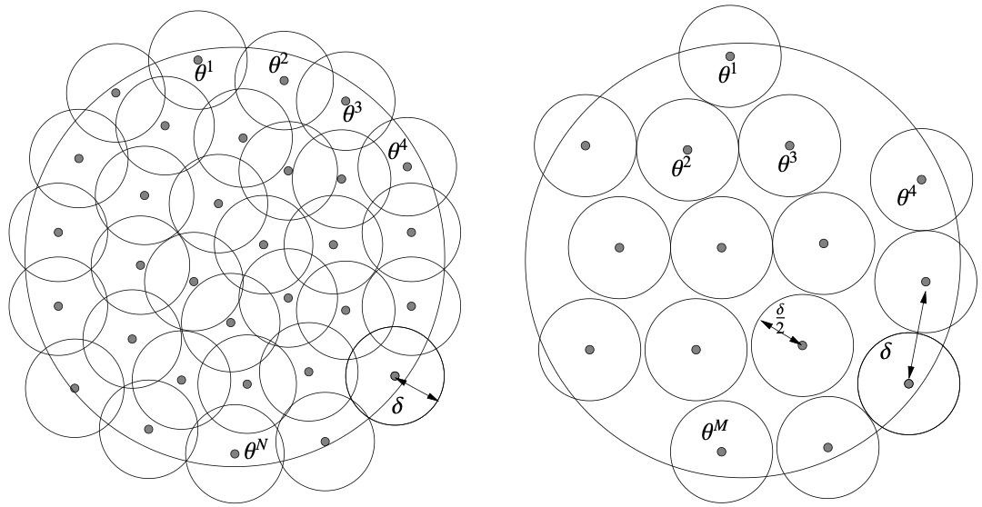
With such concepts, we can reduce the minimax estimation problem to a multiple hypothesis testing problem. We assume that the space $\left\{f(\theta )\left\lvert\right. \theta \in \varTheta \right\}$ is equipped with a metric $\rho $ and the risk function $r$ is an increasing function with respect to $\rho $: $r=r(\rho(f(\theta ),T(X)))$, as is the case for most risks. In this way, the minimax risk can be formulated as \[ \mathop{\arg \min}\limits _{T}\sup \limits _{\theta }\mathbb{E} _{\mathbf{X}}r(\rho(f(\theta ),T(X))). \] The equivalence goes as follows. Suppose $\left\{f(\theta _{1}),\dots,f(\theta _{M})\right\}$ is a $2\delta $-packing of $\left\{f(\theta )\left\lvert\right. \theta \in \varTheta \right\}$, we sample a point $Y$ from the mixture distribution $\frac{1}{M}\sum\limits _{i=1}^{M}P _{\theta _{i}}$ then we can consider which distribution $P _{\theta _{i}}$ is the source of $Y$. (This is from the definition of the mixture!) A natrual testing strategy is to look at which point in $\left\{f(\theta _{1}),\dots,f(\theta _{M})\right\}$ is the closest to $T(Y)$, and select the nearest point as the conclusion: $\hat{\theta } _{0}=\mathop{\arg \min}\limits _{\theta _{i}}\rho (T(Y),f (\theta _{i}))$. The error of such strategy is: \[ \mathbb{P}\left(\hat{\theta } _{0}\neq \theta \right)=\frac{1}{M}\sum\limits _{i=1}^{M}\mathbb{P} _{\theta _{i}}\left(\hat{\theta } _{0}\neq \theta _{i}\right)\overset{\text{(i)}}{\le } \frac{1}{M}\sum\limits _{i=1}^{M}\mathbb{P} _{\theta _{i}}\left(\rho (T(Y),f(\theta _{i}))\ge \delta \right), \] where (i) follows from the definition of $\hat{\theta }$, the definiton of the $2\delta $-packing, and the triangle inequality. Now, by the Markov’s inequality, we have \[ \sup\limits _{\theta }\mathbb{E} _{\mathbf{X}}r(\rho(f(\theta ),T(X)))\ge r (\delta )\cdot \frac{1}{M}\sum\limits _{i=1}^{M}\mathbb{P} _{\theta _{i}}\left(\rho (T(Y),f(\theta _{i}))\ge \delta \right)\ge r(\delta ) \mathbb{P}\left(\hat{\theta } _{0}\neq \theta \right)\ge r(\delta )\inf\limits _{\hat{\theta }}\mathbb{P}\left(\hat{\theta }\neq \theta \right). \] Here the infimum in $\inf\limits _{\hat{\theta }}\mathbb{P}\left(\hat{\theta }\neq \theta \right)$ is taken with respect to all possible estimators $\hat{\theta }$, and it does not depend on the choice of $T$ (recall that $\hat{\theta }$ is only the function of the observed data $Y$). Therefore, we can take the infimum over $T$ on both sides for free! \[ \text{minimax risk}\ge r(\delta )\inf\limits _{\hat{\theta }}\mathbb{P}\left(\hat{\theta }\neq \theta \right). \] This is significant! If we can calculate the RHS, then we prove that no estimator can have smaller risk!
When $M=2$, the RHS can be lower bounded by the total variation distance:
This demonstartes that, if we can find two parameters $\theta _{1}$ and $\theta _{2}$ such that $f(\theta _{1})$ and $f(\theta _{2})$ are far away ($2\delta $) in the metric $\rho$, then the minimax risk is at least $r(\delta )\cdot \frac{1-\text{TV}(\mathbb{P} _{\theta _{1}},\mathbb{P} _{\theta _{2}})}{2}$!
The example above shows that given $X _{1},\dots,X _{n}$, no matter how elaborate the estimator is, there always exists a $\mu \in \mathbb{R}$ such that the square risk is at least in the same rate as $\frac{\sigma ^{2}}{n}$. In fact, the sample mean $\bar{X}=\frac{1}{n}\sum\limits _{i=1}^{n}X _{i}$ has the risk $\mathbb{E}(\mu -\bar{X})^{2}=\frac{\sigma ^{2}}{n}$, which is minimax optimal up to a constant factor. (So do not waste your time!)
Sometimes we do not care about the exact parameter $\theta $, but rather a function of it, which means that $f$ is no longer the identity, but rather a function that maps $\theta $ to $\mathbb{R}$. In such case, the following Le Cam’s lemma of functional is useful.
Minimax Framework for Testing
Recall how we define the risk function for a testing $T$ under simple hypotheses. This definition can be naturally extended to the case of composite hypotheses by our understanding of minimax risk. For a testing function $T$ and the parameter spaces $\varTheta _{0}$ and $\varTheta _{1}$ under $H _{0}$ and $H _{1}$ respectively, we can define the risk function as \[ R _{m}(T)=\sup\limits _{\theta \in \varTheta }R(\theta ,T)=\sup\limits _{\theta \in \varTheta _{0}}\mathbb{P} _{\theta }(T(X)=1)+\sup\limits _{\theta \in \varTheta _{1}}\mathbb{P} _{\theta }(T(X)=0). \] I.e., we consider the worst case Type I and Type II errors over $\varTheta _{0}$ and $\varTheta _{1}$. However, if we do not impose any additional condition on $\varTheta _{0}$ and $\varTheta _{1}$, such minimax risk is not useful. Specifically, if we naively let $\varTheta _{1}=\varTheta \backslash \varTheta _{0}$ for some null $\varTheta _{0}$ and the whole space $\varTheta$, we will usually find that the minimax risk is always $1$, irrelevant with the testing function $T$. The reason is that the distance between $\varTheta _{0}$ and $\varTheta _{1}$ can be arbitrarily small, which means that the alternative can be as close to the null as possible, and hence leading to very bad worst-case performance.
Imagine it is the year 3026, and the global population has reached a staggering 1 trillion. Now, consider a magical hypothetical machine that takes a person and an event as inputs. It can perfectly simulate how the scenario would unfold for that specific person, all while maintaining absolute privacy with zero leakage of their true identity. You, my best friend, are tasked with finding a needle in a haystack: recognizing me among the other 1 trillion people. Your only tool is to feed candidates into this machine and observe the simulated outcomes. Could you design a foolproof strategy to identify me in the worst-case scenario?
The harsh reality is: no. No matter how brilliantly you craft the test event, a population of 1 trillion guarantees the existence of my "behavioral twin"—someone whose life experiences are so remarkably similar to mine on that specific event that they would react indistinguishably. Faced with the machine's identical outputs, you would be utterly confused, rendering your prediction no better than a random coin flip.
But the game changes entirely if we introduce a constraint. If you possess the prior knowledge that the candidate belongs to a very narrow subgroup—say, PhD students at Northwestern University—you could easily formulate an effective strategy to filter me out. Ultimately, this thought experiment captures the absolute essence of why prior knowledge of on the parameter spaces $\varTheta _{0}$ and $\varTheta _{1}$ can facilitate the testing!
Suppose there exists a distance function $d(\cdot ,\cdot )$ defined on $\varTheta $ such that $\varTheta _{1}$ is defined as all the points that are at least $\epsilon $ away from $\varTheta _{0}$: $\varTheta _{1}:=\varTheta _{1}(\epsilon )=\left\{\theta \in \varTheta : d(\theta ,\varTheta _{0})\ge \epsilon \right\}$. In this way, the risk function of $T$ is \[ R _{m}(T)=\sup\limits _{\theta \in \varTheta _{0}}\mathbb{P} _{\theta }(T(X)=1)+\sup\limits _{\theta \in \varTheta _{1}(\epsilon )}\mathbb{P} _{\theta }(T(X)=0). \] For a fixed error tolerance $\alpha $, we are interested in the smallest $\epsilon $ such that there exists a testing function $T$ with $R _{m}(T)\le \alpha $: \[ \epsilon ^{\star }=\inf\limits _{}\left\{\epsilon >0:\inf\limits _{T}R _{\epsilon }(T)\le \alpha \right\}. \] A test $T$ is called minimax rate optimal if $R _{\epsilon ^{\star }}(T)\le \alpha $.
In general, it is very difficult to find the exact value of $\epsilon ^{\star }$. Therefore, people are usually satisfied with finding a lower bound and upper bound of $\epsilon ^{\star }$ up to a constant or logarithmic factors.
We can also adopt the Neyman-Pearson framework to restrict our attention to the set of level $\alpha $ tests: \[ \mathbb{T} _{\alpha }:=\left\{T :\sup\limits _{\theta \in \Theta _{0}}\mathbb{P} _{\theta }(T(X)=1)\le \alpha \right\}. \] Then compute the minimax risk function \[ R _{\epsilon ,\alpha }(\phi ):=\sup\limits _{\theta \in \Theta _{1}(\epsilon )}\mathbb{P} _{\theta }(T(X)=0). \] The critical radius is defined similarly: \[ \epsilon ^{\star }:=\inf\limits _{}\left\{\epsilon >0:\inf\limits _{T \in \mathbb{T} _{\alpha }}R _{\epsilon ,\alpha }(T)\le \alpha \right\}. \]
How to find such testing function $T$? The following lemmas provide us some sufficient conditions.
Let $v _{0}$ be a distribution with $S _{0}:=\text{Support}(v _{0})\subset \Theta _{0}$, and $v _{\epsilon }$ be a distribution with $\text{Support}(v _{\epsilon })\subset \Theta _{1}(\epsilon )$. Let $\mathbb{P} _{\theta \sim v _{0}}=\mathbb{E} _{\theta \sim v _{0}}\mathbb{P} _{\theta }, \mathbb{P} _{\theta \sim v _{\epsilon }}=\mathbb{E} _{\theta \sim v _{\epsilon }}\mathbb{P} _{\theta }$. For any test $T =\mathbf{1} _{A}$ with some event $A \in \mathcal{F}$, we have:
where (i) is assuming $\mathbb{P} _{\theta \sim v _{\epsilon }}\ll \mathbb{P} _{\theta \sim v _{0}}$ with densities $\frac{d \mathbb{P} _{\theta \sim v _{\epsilon }}}{d \mathbb{P} _{\theta \sim v _{0}}}$ and follows from the following argument:
where again (ii) is from the Jensen’s inequality.
Recall we defined:
We have: